When it comes to neural networks, or more specifically multi-layer perceptrons, one can find in literature some contents which may be either complicated, demanding a bit of mathematical maturity, or too simplified, lacking details which would come in handy for implementation, usage, or even understanding of the mechanism as a whole.
For study purposes, I developed this tool as an additional material to be used along with contents of the literature, enabling to recreate a particular state of the network in order to inspect its behavior as a function, as well as its convergence during training, and (almost) everything else that can be studied. See in the video below an overview of this project:
I took the idea of a playground from Tensorflow’s playground, since you are free to play with multilayer perceptrons from this tool. In fact, I encourage you to make your own! It is quite a good way to explore your expertise from different perspectives. Have fun!
This project was developed in JavaScript, HTML and CSS and encompasses the implementation of the classic backpropagation training algorithm. It is entirely available at GitHub. In case you feel like adding new features and adjusting it to your needs, fork me on GitHub :).
It is important to point out that this post is a full guide of the tool. I would recommend to use it for query purposes, because a one-time reading may be a bit boring and worthless.
Open the tool in a new window or use the embedded version below for testing everything described in this guide. Below you can find a full guide of this tool divided into the following sections:
Topology tab
Everything regarding structural configuration of a model is done in this tab (you can also use the shortcut Shift+1). Changes are performed through the interface at the bottom area, and inspected at the top area.
The number of inputs, hidden nodes and outputs are adjustable through  and
and  buttons, or just change the current number and input a new one from keyboard. Layers of neurons can be removed by
  button, or added by
  button.
The activation function used in each layer is indicated by \( g(u) \) or \( u \) (click to toggle between them), being respectively a sigmoid or a linear function:
- \( g(u) = \dfrac{1}{1+e^{-u}} \)
- \( u = u \)
The configurations can be swapped between layers using the  button. In case of swapping with the input layer, only the number of nodes does swap and everything else remains in the neural layer.
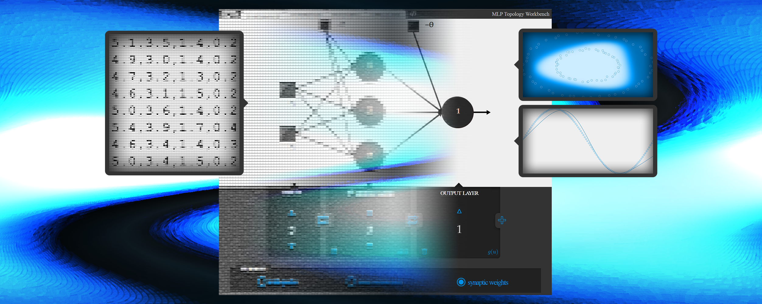
The Verbose area will be covered in the next section, since both topology and command tabs share the same interface.
Command tab
This tool was initially developed to generate commands to run the C implementation of multilayer perceptrons. So this tab (Shift+2) encompasses the commands to perform training and operation of models configured in topology tab - even though the same task can be done in this tab without visual inspection.
Right below the generated commands, there is a text area which is related to the state of the current model and will be covered in next section.
In verbose area, there are three options to be set regarding whether to verbose when running the generated command for training:
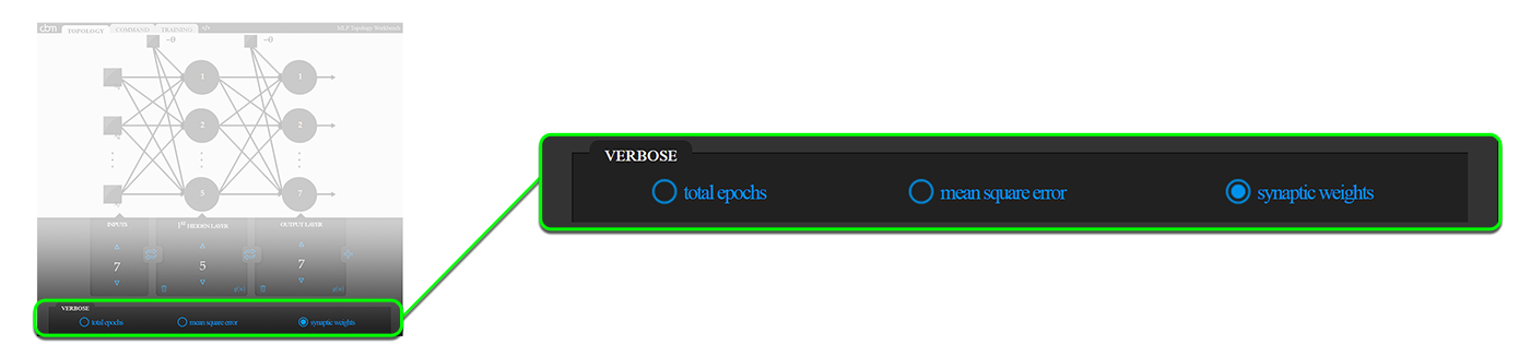
- Total epochs the number of epochs after training
- mean square error at the end of each epoch (useful for plotting)
- synaptic weights the adjusted weights after training
Train tab
Given a model previously configured at topology tab, its weights - initially random - can be changed in this tab (Shift+3) either via training, or manually.
Interactive structure
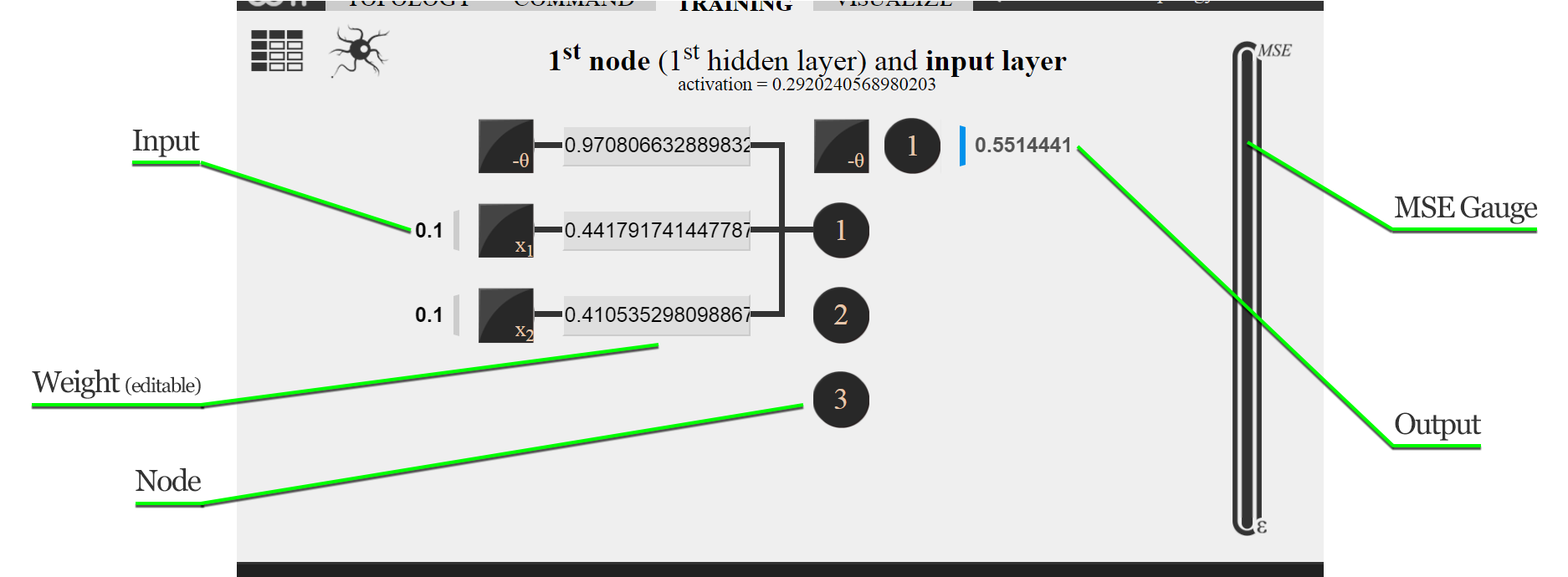
The structure displayed in this tab is interactive, so one can inspect the entire model, as well as perform changes manually.
As indicated in the image above, nodes - or neurons - are clickable, displaying (on click) its weights, which make up the connection to the previous layer. When the model is idle (i.e., when training iterations are not being performed), weights can be manually changed by modifying the value in the due text field and then pressing Return.
At any moment, regardless of the idleness, the network can be fed. Once all text fields at the left of the structure (see image above) are filled - tip: paste the input entirely in the first text field in comma-separated format, and everything is distributed to the other fields - with real-valued input, the structure is fed and the output appears at the right side.
Dataset
Before training, it is necessary to provide a dataset for the network to learn. Click  button to toggle to a text area to provide data - click
  button to toggle back. Instances must be in CSV format or a data function can be called:
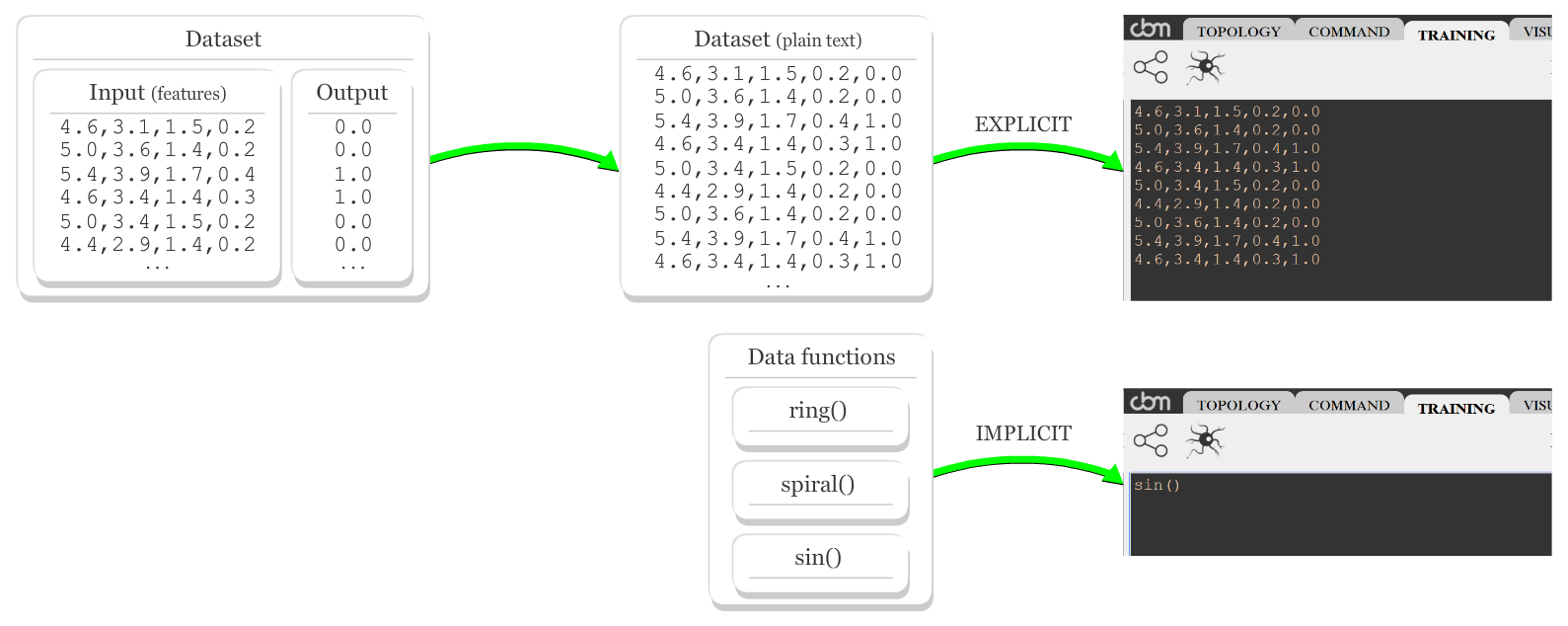
Instances must be compatible to the model IO, i.e., the number of values per instance (input and expected output) equals the total of inputs and outputs of the model. Once a new dataset is inserted, hit update parameters button.
Data functions
For didactic purposes, there are some functions to generate data points which can be used in place of explicit instances, such as ring(), spiral() and sin(), detailed below:
ring() function generates data points for binary classification in \( \mathbb{R}^3 \). Spatially, each ring of points from one class is surrounded by a bigger one from another class. Its usage is defined below:
ring();
//or
ring(points, pairs, noise, flipLabels);
where:
points:integernumber of points to be generated (both classes)pairs:integernumber of pairs of rings (one for each class)noise:decimalthe amount of noise to be addedflipLabels:booleanwhether to invert labels of data points
spiral() function generates data points for binary classification in \( \mathbb{R}^3 \). Spatially, points of both classes are arranged in a spiral pattern. Its usage is defined below:
spiral();
//or
spiral(points, twirl, noise, flipLabels);
where:
points:integernumber of points to be generated (both classes)twirl:decimalthe intensity of the twirl effectnoise:decimalthe amount of noise to be addedflipLabels:booleanwhether to invert labels of data points
sin() function generates data points for regression in \( \mathbb{R}^2 \). Spatially, points describe the behavior of the sine function. Its usage is defined below:
sin();
//or
sin(points, periods, noise);
where:
points:integernumber of points to be generated (both classes)periods:integerhow many times the period is repeatednoise:decimalthe amount of noise to be added
Training interface
At the bottom area, the adjustable parameters of the classic backpropagation algorithm are learning rate ( \( \eta \) ) and precision ( \( \epsilon \) ) as stopping criterion. Once parameters are changed, hit update parameters button.
To start training, hit iterate button. everything in the structure is updated at each iteration, and the behavior of the mean square error (MSE) along epochs can be inspected by the vertical gauge at the right. As MSE approaches \( \epsilon \), if the convergence slows down and the difference is too small to inspect visually, click the gauge area to zoom in.
Training iterations can be interrupted any time by marking interrupt option, going back to idle state. Changes of weights can be inspected between epochs, once interrupt option is marked and iterate is hit.
It is also possible to inspect changes of weights inside one epoch, as instances are presented to the algorithm, by hitting next instancec/t button, where c indicates the next i-th instance to be presented out of t instances. After iterating over all instances, an epoch is counted; if iterate button is hit when \( 1 < c < t \), the remaining instances are presented, and an epoch is counted.
In case of restarting training, hit random button, so small random values in \( [0,1] \) are attributed to all weights of the network.
Load and save states
Once a network is trained and ready to use, hit save button. It takes to the command tab and the text area below the generated commands displays the weights that make up the entire model, so it can be used in another piece of software - the color sensor project is a good example that benefits from these weights. The order of weights in relation to the nodes are defined as follows:
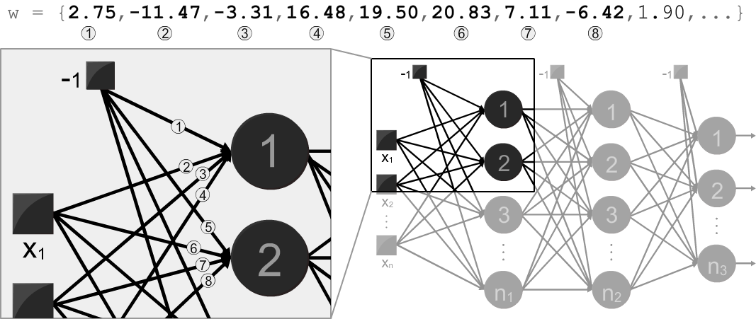
The other way around is also possible. A list of weights obtained elsewhere - a MATLAB toolbox, Tensorflow playground, or even my implementation in C language - can be applied to the network structure by pasting it in the same text area from command tab and hitting load button at train tab. Make sure to supply the exact number of weights, in the order illustrated above, necessary to make up a model with the configured structure.
The feed forward button is used when the output or activations of hidden neurons are not refreshed.
Depending of the topological configuration, the  button becomes available. More details of this feature are covered in next section.
Visualize tab
When the topology defines a function in \( \mathbb{R}^2 \) or \( \mathbb{R}^3 \), this tab (Shift+4) is enabled and ready to use. It shares the same training interface as in training tab - so the result of iterations can be observed spatially - along with visualization parameters to customize what is shown in the top area.
The size of points (from dataset) to be plotted is defined by PT SIZE and ASPECT defines the aspect ratio of the plotting area. show points button flags whether to show the points along with the output of the model. Once a parameter is changed, plot button will be marked, meaning that there are changes to be done in the visualization. Hit plot button to refresh the plotting area with the new parameters.
The default node to be visualized is the model output (i.e., the first node of the output layer). To select another node for visualization, hit button (also available in training tab, or Shift+V, regardless of the selected tab). It will take to the training tab, prompting to select another node to visualize its output in space - pass the mouse cursor over a node to see a preview of the visualization, or click to be taken to the visualize tab.
A quick note: the image of button is licensed under creative commons license. So let me give the due credits to Amelia Wattenberger.
It is important to point out that whenever a weight is changed at training tab (via training or manually), the visualization, when available, is refreshed. That said, this tool is useful to study the role of each weight in the activation of nodes - performing a manual approximation of the sin function is a good exercise - once it is possible to visualize and change the network at training tab.
Sharing
It is possible to embed this tool in an HTML page with a trained network, so the same model can be tested and used by others. Click at </> button and copy the generated HTML code. Feel free to resize the frame according to your layout, but keep in mind that minimum and maximum widths are 455 and 700 pixels.
Everything shareable is stored within the URL hash. Only the dataset is not shareable - I chose to prioritize the weights in the URL, because large datasets might get truncated.
There is also the possibility of not to embed the weights. To do so, uncheck the synaptic weights option under verbose area in topology tab, as shown below:
URL parameters
There is also the possibility to share the URL (since network weights are carried in hash) - just ignore the HTML code around the URL. The hash contains comma-separated parameters in the following syntax:
#I, N1, ..., Nm [, s | l, ..., s | l] [, eE] [, rR] [, wLIST]
where:
- UPPERCASE are numbers and lowercase are static characters
Iis the number of inputsN1, ..., Nmare the numbers of nodes (from layer1to layerm(output))[, s | l, ..., s | l]are the activation functions to use per neural layer:sfor sigmoid andlfor linear (Optional. Default iss).[, eE]is the precision \( \epsilon \). (Optional. Default isE\( = 0.01 \) ).[, rR]is the learning rate \( \eta \). (Optional. Default isR\( = 0.1 \) ).[, wLIST]is the list of weights following the order described here. (Optional. Default is a random list).LISTseparates weights with separator|
Closing remarks
The purpose of this tool is to study how this architecture of neural networks and the classic backpropagation algorithm work, as well as to share a trained model. It has a lot of limitations and therefore plenty of room for improvements. Again, fork me on GitHub if you are keen on neural networks and this tool.
This is not a data science tool - Cross-validation and preprocessing tools were intentionally not implemented, because they do not concern the main purpose. For real-life applications, Tensorflow library, Python + Scikit-learn and R are the most suitable tools.
comments powered by Disqus