Artificial Neural Networks (ANNs) and the working principle of its architectures are not subjects commonly discussed (except if you are into machine learning fields) between programmers when it comes to appliable contexts, or at least not thoroughly exploited, for instance, through examples from practical perspectives.
Divided in three sections (implementation details, usage and improvements), this article has the purpose of sharing an implementation of the backpropagation algorithm of the Multi-Layer Perceptron (MLP) architecture in C language as a complement to the therory available in the literature. Such implementation is available at GitHub.
Before approaching details of the implemented ANN architecture, it is important to point out that basic knowledge regarding MLP and backpropagation algorithm is needed. If you are new to ANNs and MLP, I would recommend you to check Freeman and Haykin references.
Implementation details
The implementation was based in this book (which is also a good reference, but only available in portuguese), coded in ANSI-C and should be compiled by GCC.
Among several variations of the backpropagation algorithm, this implementation encompasses the generalized delta-rule with the momentum term in the adjustment of weights. Both training and operation modes are implemented in the same file (check Usage section to see how to trigger each mode). Therefore, this algorithm has the following adjustable parameters:
- \( \eta \) - Learning rate
- \( \epsilon \) - Precision (stopping criterion)
- \( \alpha \) - Momentum rate
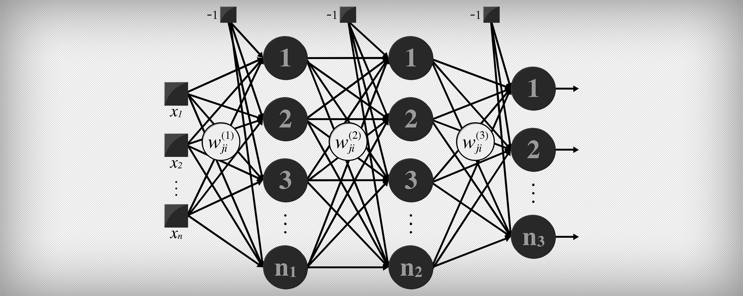
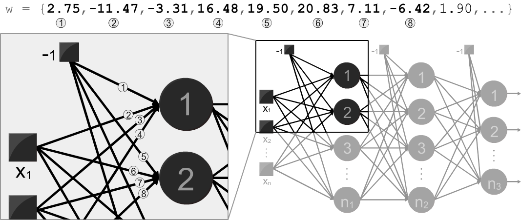
The program verboses two types of outputs (when flagged): adjusted weights and the mean square errors (MSEs) of each training epoch. The adjusted weights should be used as input of the operation mode in order to constitute the trained MLP. The weights are ordered according to the appearance of neurons in the topology (i.e., from the first neuron of the first hidden layer to the last neuron of the output layer), as indicated below:
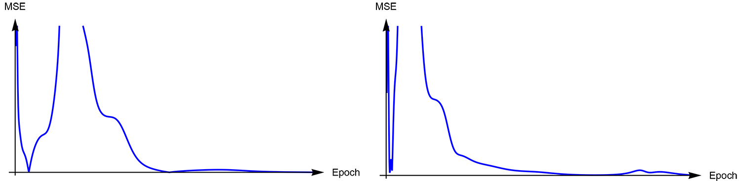
The mean square error at each epoch should be used in visualization, in order to inspect the behavior of the gradient-descent along the iterations from backpropagation algorithm, as can illustrates the plot below:
Usage
As mentioned earlier, the program has two modes: training and operation. Here is how to trigger the training mode:
cat inputFile | ./mlp -i INPUTS -o OUTPUTS -l LAYERS n1 n2 n3 [-[e | E | W]]
where:
inputFileis the dataset to be used in trainingmlpis the compiled program-iindicates the number ofINPUTS-oindicates the number ofOUTPUTS-lindicates the number ofLAYERSand its sizes-[e | E | W]everboses the number of epochsEverboses the MSE at each epochWsuppresses verbose of adjusted weights
Here is an example of a dataset to use as input in training mode, holding 6 instances; each instance consists of 2 inputs and 3 desired outputs:
6
2.0000 1.0000 1 0 0
7.0050 0.7500 1 0 0
2.0001 0.3240 0 1 0
0.0040 0.2380 0 1 0
7.0050 0.7500 0 0 1
2.0003 2.0001 0 0 1
It is important to point out in this example that numbers without a floating point represent desired outputs for classification. However, it is also possible to use floating points in desired outputs with the purpose of performing regressions or time-series predictions.
Having the output of the training mode (the adjusted weights), here is how to trigger the operation mode:
./mlp -i INPUTS -o OUTPUTS -l LAYERS n1 n2 nLAYERS -w
where:
-windicates the insertion of the adjusted weights
Runtime verbose may guide the user for inserting weights and network inputs in order to obtain the due output.
You can also use the MLP Topology Workbench either to generate commands to run the compiled program in training and/or operation modes (command tab), or as an alternative tool for training and/or operation modes:
Improvements
This implementation was focused only in algorithmic fidelity (didactic purposes), and therefore there are several improvements (from which I enumerated a few) to be done, towards an optimized and easy-to-use tool:
- Better memory management: occurrences of memory dynamically allocated could be reduced (or even replaced with static allocation approaches). No allocated memory was freed in this program (sorry, I had a tight deadline to finish this implementation)
- Operation mode (the forward step) was optimized with statically allocated memory in Neurona – a project involving MLP for AVR microcontrollers
- Parameterize (at program execution) algorithm parameters such as \( \eta \), \( \epsilon \), \( \alpha \) and and the activation function to be used.
- Implement stopping criterion by epochs (also parameterizable).
- Append a new parameter to set a random seed, so outputs/outcomes can become reproductable.
- Input buffer reading improvements, enabling batch-like feed for several instance in operation mode.
Fork me on GitHub if you’re keen on MLPs and ANNs and liked this project :)
comments powered by Disqus